Changelog
Indicator: Virtual Gauge volume level estimates
Inputs: JAXA ALOS World 3D-30m (AW3D30)
Methodology: Volume level estimates are arithmetically calculated using elevation readings from the ALOS digital elevation model (DEM) and established full reservoir levels. Established reservoir levels at full storage capacity determine the maximum altitude in meters above sea level which masks elevation readings above the maximum, leaving only values at or below the maximum altitude and forming the full extent of the reservoir at full storage capacity. The masked elevation layer is vectorized, summarized by the count of each cell value (altitude in meters above sea level), and extracted as a spreadsheet of each elevation reading and its corresponding count within the reservoir extent.
The extracted data is converted from vertical (long) format to horizontal (wide) to create an index table with meter-by-meter volume estimates. To convert the table, all pixel counts are first added together- encapsulating the total amount of pixel in the entire reservoir at full water supply level. Then pixels are subtracted from the total amount at each elevation reading- resulting in the total amount of pixels at each elevation. These pixel count values are multiplied by the cell size of the original ALOS DEM- 900 meters (30m x 30m), which results in the total volume estimate at each water level, by meter. The total reservoir volume is calculated by summing all the meter-by-meter volumetric readings together. The sum of the readings is the total volume at the maximum water level and finding the difference between the total volume at maximum water level and the volume values at each meter below the maximum water level creates a dataset depicting water volume changes at each one-meter increment.
The project team has derived look-up tables detailing reservoir volume at one-meter increments for all dams monitored on the Mekong which correspond to altimetry estimates of reservoir levels. Volume readings is used to estimate dead and active storage levels. Dead storage is the volume of water held behind a dam that will likely never flow downstream. This water is likely permanent stored upstream. Active storage is water that is available for hydropower production or other uses and is likely or has potential to flow downstream through the dam. Active storage is calculated by finding the difference between the total volume reading for a given week and the known or estimated dead storage level for each reservoir.
Indicator: Virtual Gauge meters above sea level estimates (altimetry)
Inputs: Sentinel-1 SAR GRD, Sentinel-2 MSI, JAXA ALOS World 3D- 30m (AW3D30)
Methodology: The process below details how the Stimson Center determines altimetry estimations for its virtual gaugues. We draw from existing literature to detect and map the extent of surface water using satellite imagery observations. Many methods described include the use of visible and Near-Infrared bands from multispectral satellites to construct indices that can be used to detect bodies of water, including the Normalized Difference Water Index (NDWI), the Modified Normalized Difference Water Index (MNDWI), and the Normalized Difference Vegetation Index (NDVI).
However, these methods rely on optical images and for regions in the world where cloud contamination is common, like Southeast Asia during the wet season (broadly June through October), so researchers must look to other remote sensing products like Synthetic Aperture Radar (SAR). SAR products, like the Sentinel-1’s C-band SAR, transmit radio waves sequentially and receive and record its echoes to create landscapes. These readings can “pierce” through cloud contamination and record readings day or night, making the use of these remote sensing products highly useful for tracking water level changes in cloud-heavy regions.
Literature on using Sentinel-1 to monitor water levels temporally are extensive. Bioresita et al. propose a fully automatic method to detect rapid flood and surface water mapping over large areas and demonstrate the use of Sentinel-1 for water/flood detection by leveraging the satellite’s high spatial resolution and short temporal baselines to capture temporal and spatial water level dynamism. Similarly, Pham-Duc et al. apply a neural network classification trained on optical data to detect and monitor surface water using Sentinel-1 SAR in Cambodia and the Mekong Delta and show the efficacy of using SAR data in tropical regions during the wet season. Building on those and other similar work, Gulács and Kovács present an analytical method using the Google Earth Engine (GEE) cloud-processing platform to capitalize on the time-consuming geoprocess required in big data analysis. Shifting to cloud processing platforms can speed up processing, expand the scaling potential, and provide a shared platform for researchers around the world.1https://ieeexplore.ieee.org/abstract/document/7565634 and https://www.mdpi.com/2072-4292/10/5/711/htm.
The process to estimate water (reservoir and river) altimetry levels in meters above sea level at the Mekong Dam Monitor’s virtual gauge sites is derived from Gulács and Kovács and modified to meet the platform’s needs using GEE’s preprocessed Sentinel-1 SAR GRD dataset. In addition to keeping existing processes like normalizing the incidence angle, cleaning the data using the Refined Lee speckle filter, and clustering using WEKA K-Means, we modified code to process images at a rate dependent on the orbital interval of the satellite for each reservoir’s area of interest that varies based on the year and area (5-12 days). The research team identifies water clusters with the classified image (see image 1). The Google Earth Engine code can be found here.

This result is then exported to Esri’s ArcGIS Pro for further analysis. Sentinel-2 MSI is used as additional support for certain periods and locations where Sentinel-1 data is missing or of lower quality.
After reservoir shapes are transferred from GEE to ArcGIS, the reservoir extent polygon is isolated from any extraneous polygons that have been captured in the classification using a query of the shapes’ area. Next, generated lines that clearly follow the observed shoreline and elevation contours are selected for processing by creating a polygon to clip out those sections (image 2). Sections of shoreline that are distorted due to shadows, irregular features, or poor satellite angles are therefore eliminated from processing (image 3).


The clean shorelines are rasterized so elevation values can be extracted from the digital elevation model (JAXA ALOS World 3D- 30m) with map algebra. The shoreline elevation values are generalized with median filtering to reduce the incidence of outlier observations. Finally, the original shoreline raster is used as the feature zone input for zonal statistics, and the shoreline with median filtering is input as the value raster, which returns the mean elevation of the shoreline for a single period of observation.

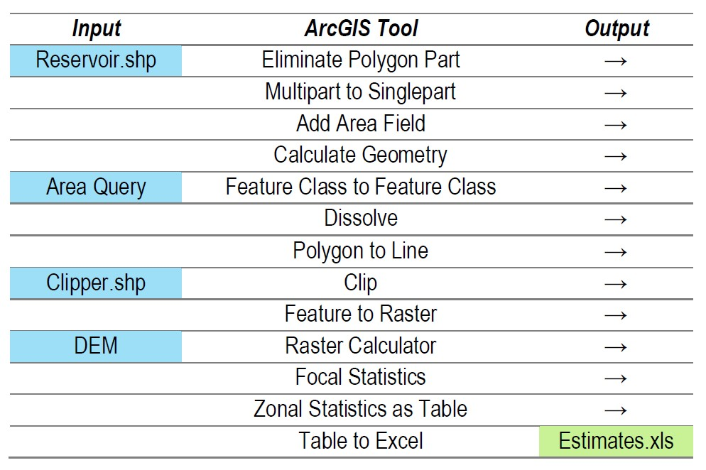
The entire analysis process in ArcGIS Pro is automated with ArcGIS Model Builder (image 4). The user must only input the following to return an elevation estimate: GEE reservoir shapes, DEM, area query, and clipper polygon for desired shorelines. (image 5)
These mean elevation estimates then go through a final checking and validation stage using observations from high-resolution satellite imagery such as the input images from Sentinel-1 SAR GRD or Sentinel-1 MSI or other satellite image service. This final stage includes comparing current estimates to past estimates to check for outliers and to determine a normal maximum level for the reservoir and regular low level for the reservoir. This final stage also confirms whether comparative outlines are actual extreme flood or drawn-down events. This final stage also checks whether anomalous fluctuations observed in the raw data across the time series is actually present on the satellite imagery or is a result of noise not removed during the processes described above. Prior to this validation stage, we believe the raw data collection produces a mean elevation shoreline typically within 5 meters (+/- 2.5 meters) of actual reservoir levels. The final stage improves the accuracy of the estimates to within about 2 meters (+/- 1 meter) of actual reservoir level.
The aforementioned error results were confirmed by a blind validation process conducted through an analysis of reservoir levels across the year of 2019 for the Nam Khan 2 dam in Laos (image 6 below). EDL-Gen, a partial owner of the Nam Khan 2 dam, produces daily meters above sea level readings for the Nam Khan 2 dam reservoir. Below is a comparative result of the model described above versus actual reported data of Nam Khan 2 reservoir levels (masl). The Nam Khan 2 dam was chosen as a validation test case due to its relatively mountainous location and location in the middle portions of the Mekong Basin.

Below is a second iteration of the model validation process, this time conducted in Chiang Saen and compared to actual Mekong River Commission gauge data for Chiang Saen. This demonstrates the process’s ability to generate estimates along a river where there is no reservoir or dam nearby (image 7).

Indicator: Virtual Gauge Image Comparison
Inputs: Sentinel-1 SAR GRD, Sentinel-2 MSI
Methodology: Images used in the Virtual Gauge Image Comparison were captured and exported through the Google Earth Engine (GEE) cloud processing platform. Images were taken from either Sentinel-1 SAR GRD or Sentinel-2 MSI, providing both a landscape and optical perspective of each area of interest. Images derived from Sentinel-1 were processed to correct for incidence angles and backscatter issues. Sentinel-2 images are presented using optical bands (RGB) and provide a top-of-atmosphere view of the areas of interest.
Indicator: Virtual Gauge Operations Curves/Time Series
Inputs: Virtual Gauge meters above sea level readings time series data
Methodology: This indicator is compiled by arranging virtual gauge meters above sea level (masl) readings as a time series across a 12-month period. Numerous 12 month periods can be visualized to compare how dam operations change or how the hydrological cycle of the river changes at respective impact areas. See “virtual gague meters above sea level readings” above for information on how this indicator is determined and validated.
Indicator: Virtual Gauge Shape (of reservoir)
Inputs: Sentinel-1 SAR GRD
Methodology: Shapes are created using a compilation of Sentinel-1 images from a period of time where water levels were stable as determined by the size of a reservoir’s surface area. Images were processed and cleaned by normalizing the incidence angle and through the Refined Lee speckle filter. Processed images were clustered and classified by the research team. Shapefiles created through the classification process are exported to Esri’s ArcGIS Pro for further processing and analysis.
Indicator: Cascade analysis (reservoir level, water flow, electricity production)
Inputs: Virtual Gauge meters above sea level readings (see above), Chiang Saen Natural Flow Model data (see below), Mekong River Commission gauge data for Chiang Saen Station, descriptive statistics about dams in cascade (wall height, normal maximum reservoir level)
Methodology: Cascade analysis and visualization is produced through bringing numerous Mekong Dam Monitor platform indicators together into a single visualization. Weekly or monthly virtual gauge meters above sea level readings are determined as a portion of normal maximum reservoir height and inputted as a reservoir shape (height) in the cascade visualization for all dams in the cascade. A reservoir change arrow denotes direction of reservoir change for current report period compared to the previous report period. Qualitative descriptors (minimum, slow, normal, fast) are assigned to water flow and electricity production by assessing how reservoir levels change from period to period and through how water moves through the cascade from the upstream to the downstream. For example, if a reservoir level increases relative to the previous report period, a qualitative indicator of reduced flow and reduced hydropower production is assigned. Increased flow and increased hydropower production is assumed if a reservoir is draining. Normal flow and normal levels of hydropower production are assigned typically if the reservoir is mostly full across a long period of time or stays at one level across a long period of time. Eyes on Earth Natural Flow Model and MRC gauge measurements are simply reference points for the user to gain better understanding of how upstream operations are affecting downstream outcomes. Validation: Qualitative descriptors are decided upon a weekly basis by the entire research team. The research team reaches consensus on assigning descriptors by observing changes from one period to another as well as through looking at other data (such as the wetness index/anomaly and precipitation) available on the platform.

Indicator: Chiang Saen Natural Flow Model
Inputs: Wetness Index Data (see below), Mekong River Commission gauge data for Chiang Saen
Methodology: As an effort to identify the amount of water flowing into the main stem of the upper Mekong basin, the Eyes on Earth team uses the satellite derived (surface wetness product) as the data source to detect the amount of liquid water accumulating in the upper Mekong basin. (see Wetness Index indicator methodology below for more information). The MRC gauge serves to calibrate river flow data, measured at Chiang Saen. Flow measurements are averaged into monthly mean values from January 1992 through November 2020 (period of record). The satellite derived wetness values are also averaged into monthly mean values for the upper Mekong basin over the same period of record.
We derive a regression equation based on these two data sets to quantify their relationship: namely, measuring fluctuations of flow at the Chiang Saen gauge. The period between 1996 through 2001 serves as the calibration period for the model because this period is the best representative period of natural flow during the period of the period. The relationship forms a quadratic regression model, which explains 90% of the natural variability of river flow at the gauge, and results are significant at the 0.999 confidence level. The 72 observations provided more than sufficient degrees of freedom (69) and independence to fulfill the requirements of the central limit theorem. The signal-to-noise ratio is high, since the Mekong has a strong annual cycle in flow during the calibration period, which allows the development of the stable and precise model, as demonstrated by an R square value of 0.90.
The relationship is not simple, nor is the model, as it uses a quadratic formula and a lag time to simulate natural flow originating from the upper Mekong Basin. The non-linear term is based on the fact that when there is a small quantity of water near the surface, it is largely held in the soil and does not flow towards a river. However, as the wetness value increases, a higher percentage of the water flows towards the river. When the soil is saturated, all the water flows downstream or raises the groundwater level. Therefore, the relationship between the wetness index and river flow is non-linear. Moreover, it takes considerable time for liquid water at the surface to either work its way through the groundwater or percolate through the soil, as water moves toward the streams that feed the main stem of the Mekong river.
Due to this time lag, the optimum model weights the wetness from three months earlier as 10% of the fluctuation of flow measured at the Chiang Saen gauge. Two months earlier has a weight of 20%. One month earlier has a weight of 60%. The wetness value from the concurrent month has a weight of 10%. This lagged relationship has the best explanatory skill and the smallest errors. The Eyes on Earth team validated the accuracy and stability of the model, using independent years 2005 through 2008 (period of time before a major dam and reservoirs were established in the upper basin). In order to analyze the relationship between predicted and measured flow, we plotted the two curves over the period of record, along with their difference field over the period of record. These methods are further explained in this working paper published in 2016.

Indicator: Vientiane Natural Flow Model
Inputs: Wetness Index Data (see below), Mekong River Commission gauge data for Chiang Saen
Methodology: Methods used to generate a natural flow model for the Vientiane gauge are similar to the Chiang Saen natural flow model explained above. The Eyes on Earth team uses MRC data from the Vientiane gauge as the calibration of river flow data at Vientiane. The flow measurements are averaged into monthly mean values from January 1992 through November 2020 (period of record). The satellite derived wetness values are also averaged into monthly mean values for the Mekong Basin extending down to Vientiane over the same period of record. The regression equation used these two data sets to quantify their relationship: namely, measuring fluctuations of flow at the Vientiane gauge. Similar to the Chiang Saen gauge, 1996 through 2001 serves as the best available calibration period.
The quadratic regression model explained 87% of the natural variability of river flow at the gauge, the results are significant at the 0.999 confidence level. The 72 observations provide more than sufficient degrees of freedom (69) and independence to fulfill the requirements of the central limit theorem. The signal-to-noise ratio is high, since the Mekong basin at Vientiane has a strong annual cycle in flow during the calibration period, which allows the development of the stable and precise model, as demonstrated by R square value of 0.87.
The relationship uses a quadratic formula and a lag time to simulate natural flow originating from the upper Mekong Basin. Due to this time lag response at Vientiane, the optimum model weighted the wetness from three months earlier is 10% of the fluctuation of flow measured at the Chiang Saen gauge. Two months earlier has a weight of 20%. One month earlier has a weight of 40%. The wetness value from the concurrent month has a weight of 30%. This lagged relationship has the best explanatory skill and the smallest errors. In order to analyze the relationship between predicted and measured flow, we plotted the two curves over the period of record, along with their difference field over the period of record. These methods are further explained in this working paper published in 2016.
.

Indicator: Wetness Index (anomaly)
Inputs: Channel Measurement Special Sensor Microwave Imager flown aboard the Defense Meteorological Satellite Program and an algorithm which translates the signal into a derived surface wetness product.
Methodology:
Wetness Index begins as microwave satellite measurements collected at various frequencies and polarizations (Basist et al. 2001). A complex hierarchical decision tree compares the satellite observations to ground truth to calculate the magnitude of liquid water near the surface. The Basist Wetness Index (BWI) is derived from a linear relationship between channel measurements, where the change of emissivity, Δε, is empirically determined from global SSM/I measurements. Specifically, the greater the wetness value, the larger the cold bias between the observed surface temperature and the observed channel measurements (Williams et al. 2000).
It became apparent that satellite derived surface wetness observation throughout the world (even under cloud cover) is a useful tool for monitoring land surface processes and can be used to identify the amount of liquid water in the radiating land surface. The wetness product contains information from all sources of wetness: soil moisture, liquid water, snow melt, precipitation, evapotranspiration, bogs, and vegetation. Simply stated, the wetness index is highly sensitive to any source of liquid water near the near, including dew. The Eyes on Earth team has developed a long term climatology for 1992 to 2018 from which anomalies (variation from normal) can be developed. Maps and data sets of these anomalies are presented each week on the Mekong Dam Monitor, and they serve as an effective tool to assess changing surface conditions, which impact river and soil moisture throughout the basin. The integration of all this information into the Wetness Index is what makes the natural flow model based on a single variable explained above possible.

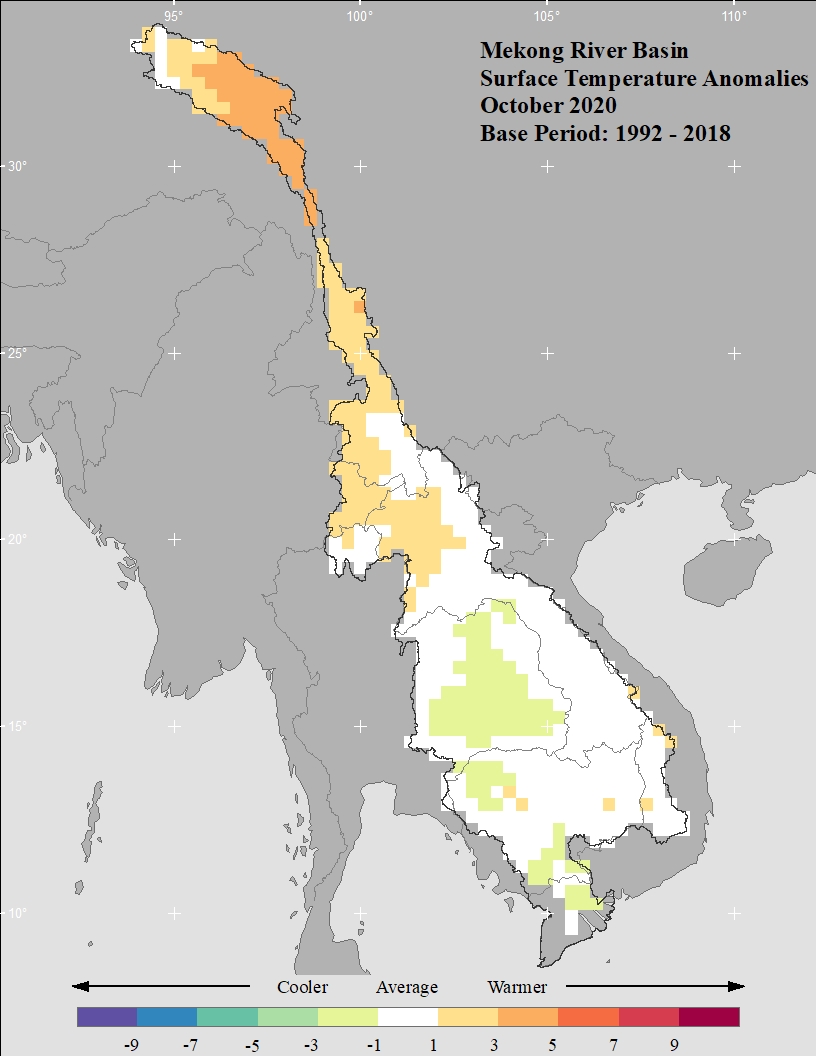
Indicator: Temperature anomaly
Inputs: Channel Measurement Special Sensor Microwave Imager flown aboard the Defense Meteorological Satellite Program and an algorithm that translates the signal into a derived surface temperature product.
Methodology: The technique to derive surface temperature from SSMI channel measurements uses a set of equations that identify various surface types and make corresponding dynamic emissisity adjustments. This allowed estimation of the shelter height temperatures from the seven channel measurements flown on the SSMI instrument. Data from first order in situ stations over the eastern half of the USA were used to calibrate the temperature signal and to inter-calibrate among satellites. The results show that the observational difference between the in situ point measurements and the SSM/I derived areal temperature values is about 2 degrees celsius with statistical characteristics largely independent of surface type. High resolution monthly mean anomalies generated from the U.S. cooperative network served as independent verification over the same study area. Verification work determined that the standard deviation of the monthly mean anomalies is 0.76 degrees celsius in each 1 degree by 1 degree grid (Williams et al. 2000).
In an effort to derive surface temperature from satellite observations, it is necessary to overcome the reduction of emissity due to water near the surface. Consequently we developed a sophisticated technique to identify the magnitude of the water and filter its influence. Specifically, in order to detect land surface temperatures, this bias must be removed. In the process of accurately identifying the emissivity reduction associated with liquid water surface and removing its effect on reduction in temperature observations, we were able to accurately identify the temperatures near the surface under most surface types and sky cover conditions. We have developed a long term climatology for 1992 to 2018 from which temperature anomalies (variation from normal) can be developed. Maps and data sets of these anomalies are presented each week, they serve as an effective tool to assess changing surface temperatures, which impact soil moisture, evapotranspiration, planting and harvest conditions throughout the basin.
Indicator: Snow Cover anomaly
Inputs:Channel measurement Special Sensor Microwave Imager flown aboard the Defense Meteorological Satellite Program and an algorithm that translates the signal into a derived snow cover product.
Methodology: A decision tree, containing various filters, is used to separate the scattering signature in the special Sensor channels flown on the DMSP satellites. These filters discriminate the signal of snow cover from other scattering signatures. In an iterative approach, problem areas and unique snow cover structure (various crystalline forms) are identified. When required, additional filters are applied to separate the snow cover signal from other features that are also scatterers in the microwave spectrum. Generally, these spectral characteristics depend on the volumetric properties of the material that is passively emitting microwave signals into the space. The polarization characteristics in the microwave frequencies flown on the SSMI instrument serve as valuable filters, and are excellent discriminators of surface characteristics, which helps separate snow cover from other surface features (Grody and Basist 1996). The final decision tree is an objective algorithm to monitor the global distribution of snowcover from the SSMI channel measurements. Snow cover products derived from satellite instruments measurements in the visible spectrum are compared against the snow cover products derived from the microwave spectrum (Basist et al. 1998). We have developed a long term climatology from 1992 to 2018 from which snow cover anomalies (variation from normal) can be developed. Maps and data sets of these anomalies are presented each week, they serve as an effective tool to assess changing snow cover and glacial melt on the water resources in the basin.

Indicator: Precipitation anomaly
Inputs: Global Precipitation Measurement (GPM)
Methodology: Precipitation anomaly data and its derived maps are created through the processing and analysis of data from the Global Precipitation Measurement (GPM), an international satellite mission launched by NASA and JAXA. Monthly data is collected using Google Earth Engine (GEE), which is then compared to the median value from 2000 to present.

Indicator: Basin-wide dams and status
Inputs: Mekong Infrastructure Tracker power generation geodatabase of dams for the Mekong Basin.
Methodology: Access this link to Mekong Infrastructure Tracker methodology page
In order to provide a comprehensive picture of state of dam development in the Mekong Basin, this tab provides data on the current condition of planned, operational, and under construction dams in the Mekong Basin. Clicking on each dam icon will provide descriptive information about each dam including its status, year of completion, generation capacity, and information about the project’s owners, financiers, and construction companies/suppliers. News links and status updates will be done on a quarterly basis.


Current Geopolitics Shift Deep-Sea Mining Debates